In this post, I’d like to muse about the visualizations that are used when thinking about math, and how they can become quite beautiful as well as useful
When adding 


This post is supposed to illustrate that visual thinking remains useful in more advanced math, especially mathematical analysis (real analysis, complex analysis, functional analysis, differential equations) which deals with objects you can imagine embedded in space (that is, with a metric). It’s just that the pictures become more and more rarely taught. That means it takes a motivated attitude and some patience, because often in classes you generally have to figure it out for yourself.
I’ve found that it is worth the effort. This post will give a couple of examples using partial differential equations (PDEs). PDEs are very useful in engineering disciplines, yet it is not often taught how to picture the solution.
For example, let’s consider Laplace’s equation.

In classical physics, the electrical potential 
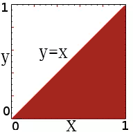
Say we want to know the potential in a long square pipe (a square cylinder), and we are given boundary conditions that specify the potential of each of the four sides. We can visualize what this equation is saying. The equation is local and it says that at every point of the domain, the x-curvature of the potential must cancel with the y-curvature of the potential.
I picked some boundary conditions (parabolas on the ends and constants at the side) and plotted the solution for
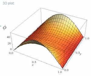
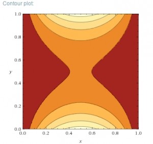
We can visually check that the curvature in x and y are equal and opposite at every point. Note how the solution looks like a stretched membrane. That’s because a stretched membrane also follows also follows Laplace’s equation. The solution is essentially the simplest surface you can draw that will connect the boundaries. If you can picture gluing an elastic sheet to those boundaries, you can picture the solution to Laplace’s equation.
Quantum probability current
In the example of the Schrödinger equation, the rate of change of the Hilbert state vector is determined by the Hamiltonian operator.

Operators and state vectors are abstract and we are sometimes interested in the positions basis specifically, since let’s face it, space seems to be a dominant aspect of reality. For the 1-dimensional problem of a free particle in the position basis we get the partial differential equation:


Animation created with Python and ImageMagick
Now for the last part of this example, let’s look at the probability current. Usually when this is taught it seems to be a terribly opaque abstract construct. The probability current 


It is difficult to picture what this equation is telling us! And yet wiki pages and textbooks* everywhere just state it and move on, letting the student grapple with it in the problem set. Let us stubbornly pursue a better picture. Using the polar form of the complex quantity 

The fraction of probability leaving location x is simply the derivative of the phase. In three dimensions, 
Using the example of the corkscrew above, simply stated, the angle 
Here are other relations that are useful for visualizing these single-particle dynamics. Here I use shorthand for the derivatives so 


The point of this post is just some examples of looking at partial differential equations to get a feeling for what the solutions look like. Locality of a PDE is a powerful property, something that college students often don’t appreciate in the standard science/engineering curriculum. My intuition dramatically increased once I began writing numerical codes to solve PDEs.
So I encourage the new mathematical scientists and engineers out there, don’t be afraid to break down your math problem and visualize it! It is worth the effort.
*Nearly all textbooks I have found stop at the abstract form of the probablility current. I eventually found however that Sakurai Modern Quantum Mechanics 1994 contains the same simple equation for