In this post, I’d like to muse about the visualizations that are used when thinking about math, and how they can become quite beautiful as well as useful
When adding  , many people imagine stacking blocks and then see
  spilling over the
  mark. This visual thinking made the answer seem “obvious” after doing it many times. When doing calculus, simple picture tricks are taught less often. If confronted with
  we might quickly follow the memorized rule (from the fundamental theorem of calculus) that you add
  to the exponent and divide by that number.
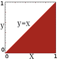
  . But one can also remember that integration finds the area under a curve. With a picture in mind like the one below, we know that the red line cuts the unit square into two parts, each with area
  . The visual understanding will sometimes be a useful tool.
This post is supposed to illustrate that visual thinking remains useful in more advanced math, especially mathematical analysis (real analysis, complex analysis, functional analysis, differential equations) which deals with objects you can imagine embedded in space (that is, with a metric). It’s just that the pictures become more and more rarely taught. That means it takes a motivated attitude and some patience, because often in classes you generally have to figure it out for yourself.
I’ve found that it is worth the effort. This post will give a couple of examples using partial differential equations (PDEs). PDEs are very useful in engineering disciplines, yet it is not often taught how to picture the solution.
For example, let’s consider Laplace’s equation.

In classical physics, the electrical potential  satisfies Laplace’s equation in three dimensions everywhere in space that there is no electric charge.
Say we want to know the potential in a long square pipe (a square cylinder), and we are given boundary conditions that specify the potential of each of the four sides. We can visualize what this equation is saying. The equation is local and it says that at every point of the domain, the x-curvature of the potential must cancel with the y-curvature of the potential.
I picked some boundary conditions (parabolas on the ends and constants at the side) and plotted the solution for below using Wolfram Alpha.
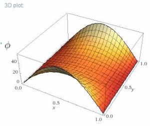
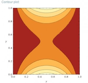
We can visually check that the curvature in x and y are equal and opposite at every point. Note how the solution looks like a stretched membrane. That’s because a stretched membrane also follows also follows Laplace’s equation. The solution is essentially the simplest surface you can draw that will connect the boundaries. If you can picture gluing an elastic sheet to those boundaries, you can picture the solution to Laplace’s equation.
Quantum probability current
In the example of the Schrödinger equation, the rate of change of the Hilbert state vector is determined by the Hamiltonian operator.

Operators and state vectors are abstract and we are sometimes interested in the positions basis specifically, since let’s face it, space seems to be a dominant aspect of reality. For the 1-dimensional problem of a free particle in the position basis we get the partial differential equation:

 is a complex field, in the sense that it has both real and imaginary components, and we can… really imagine it. The equation can be decomposed into two equations, one for the real part and one for the complex part of
  , and we can plot it using a polar plot at each value of x. Again, the equation is local and says that the curvature is what matters. Where the curvature of the real part is positive, the imaginary part will grow. Where the curvature of the imaginary part is positive, the real part will shrink. If initially the field looks like a plane wave
  where
where  is a constant, the equation is telling us the corkscrew will turn.
Animation created with Python and ImageMagick
Now for the last part of this example, let’s look at the probability current. Usually when this is taught it seems to be a terribly opaque abstract construct. The probability current  is essentially the quantity that, together with the probability
  , satisfies the continuity equation
  when
when  follows the Schrödinger equation. In one dimension it is

It is difficult to picture what this equation is telling us! And yet wiki pages and textbooks* everywhere just state it and move on, letting the student grapple with it in the problem set. Let us stubbornly pursue a better picture. Using the polar form of the complex quantity  and working through a little math we get an equation for the flow of that is much simpler to picture.

The fraction of probability leaving location x is simply the derivative of the phase. In three dimensions,  which is saying that the probability current is just “flowing uphill” of the phase. That’s what the phase of a wave function has always meant, in case, like me, you weren’t told. This simpler version gives insight that might even be useful to a new wave of physics students.
Using the example of the corkscrew above, simply stated, the angle  of the corkscrew increases constantly to the right, so our equation tells us there is uniform probability current to the right.
Here are other relations that are useful for visualizing these single-particle dynamics. Here I use shorthand for the derivatives so  and
and  . In the following, ignore the constant factors of
  which could be swallowed into the definition of the phase. The phase at a point x will decrease if it is sloped and it will increase due to curvature of A
  . Meanwhile the amplitude A at the point x decreases from phase curvature or from slopes
  . The probability increases from amplitude curvature (“smoothing out humps”) and decreases wherever the phase is sloped
  . Hope this helps you picture some quantum dynamics.
The point of this post is just some examples of looking at partial differential equations to get a feeling for what the solutions look like. Locality of a PDE is a powerful property, something that college students often don’t appreciate in the standard science/engineering curriculum. My intuition dramatically increased once I began writing numerical codes to solve PDEs.
So I encourage the new mathematical scientists and engineers out there, don’t be afraid to break down your math problem and visualize it! It is worth the effort.
*Nearly all textbooks I have found stop at the abstract form of the probablility current. I eventually found however that Sakurai Modern Quantum Mechanics 1994 contains the same simple equation for as above.
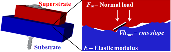
 , the root-mean-squared slope of the surface, determines the microscopic contact area, for an applied force on the block,
  , made of material with Young’s modulus
  .
.
 , where
  is the confining pressure,
  is the material’s contact modulus,
  is the effective Poisson ratio,
  is a dimensionless constant with value about 2.2.

 ) approaches zero as the log of applied force
  . When
  and
and  , the result collapse for different symbols, corresponding to continuum and atomistic simulations with varying roughness parameters. The lowest forces correspond to effects from our simulations having limited size, while the regime with slope
  corresponds to an exponential relationship between applied pressure and the gap size.
 where
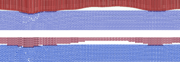
where  is the apparent surface area. As a result, the stiffness of the interface is
  . The stiffness of the interface is extremely low when there is no confining pressure, and so the surface roughness dominates the mechanical response of the whole two-block system.