Essentially all materials have rough surfaces at small scales. This can be a problem for engineers designing electrical contacts, thermal contacts, or seals to prevent leaks, since the roughness creates gaps between the two contacting surfaces. By increasing the pressure, the two solids can be forced closer together, reducing the gaps somewhat, but some space between the surfaces usually still remains.
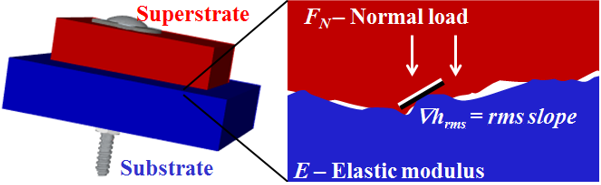
 , the root-mean-squared slope of the surface, determines the microscopic contact area, for an applied force on the block,
  , made of material with Young’s modulus
  .
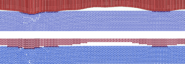
.Work with Mark O. Robbins quantified how surprisingly resilient the gaps are, and how important they are in determining the contact properties. To analyze the problem, we had to overcome technical challenges related to the large range of length scales of random-rough geometry on typical material surfaces, usually millimeters down to atomic scales. The rough geometry can be modeled using the mathematics of random (self-affine) fractals. Large-scale parallel processing on a computing cluster is required to simulate and analyze contact between many random realizations of rough 3D cubes of length 1000 atoms on a side. We worked with Lars Pastewka to write C++ code for GPUs to do fast simulations using lattice Greens functions and continuum-elastic Greens functions, which will be described in a later post.
 . However, must be very large to enter the limiting plastic regime, where the contact area is the applied force over the material yield stress.
We found that the large-scale features of the material’s surface get flattened more easily, but the small-scale roughness cannot be squeezed away even at considerable pressures; we found that the fraction of the surface that is in contact is well-defined and at common pressures is less than 20%. Within this regime the fractional contact area obeys a simple law: 


We considered this problem with both continuum-scale and atomic-scale simulations. We found that the continuum results can often be applied to small scales, meaning that continuum analyses are often appropriate for nanotechnology applications[2]. At the atomic-scale, the concept of contact area gets replaced by the number of atoms that exert repulsive forces on the other surface. However, for very rough or crystalline surfaces, atomic-scale plasticity causes the value of

 ) approaches zero as the log of applied force
  . When is normalized by surface rms height
  and is normalized by the product of macroscopic contact area and contact modulus,
  , the result collapse for different symbols, corresponding to continuum and atomistic simulations with varying roughness parameters. The lowest forces correspond to effects from our simulations having limited size, while the regime with slope
  corresponds to an exponential relationship between applied pressure and the gap size.
Even if the contacting materials are very stiff, they can seem much less so because of the gap from roughness at the contacting surface; the rough topography can be compressed more easily than the solid material. For both atomic and continuum analyses, the average gap width, 


References:
Chapter 5 of my thesis (papers in preparation)
Sampling of the related work that helped build up this picture:
 Hyun, S., et al. "Finite-element analysis of contact between elastic self-affine surfaces." Physical Review E 70.2 (2004): 026117.
 Pei, L., et al. "Finite element modeling of elasto-plastic contact between rough surfaces." Journal of the Mechanics and Physics of Solids 53.11 (2005): 2385-2409.
 Cheng, S. & Robbins, M.O. "Defining contact at the atomic scale."  Tribol Lett (2010) 39: 329. https://doi.org/10.1007/s11249-010-9682-5
 C Yang and B N J Persson 2008 J. Phys.: Condens. Matter 20 215214 http://iopscience.iop.org/article/10.1088/0953-8984/20/21/215214/
 Persson, B. N. J. "Relation between interfacial separation and load: a general theory of contact mechanics." Physical review letters 99.12 (2007): 125502.
 Mo, Yifei, Kevin T. Turner, and Izabela Szlufarska. "Friction laws at the nanoscale." Nature 457.7233 (2009): 1116.
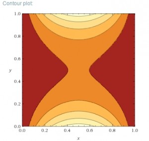
 , many people imagine stacking blocks and then see
  spilling over the
  mark. This visual thinking made the answer seem “obvious” after doing it many times. When doing calculus, simple picture tricks are taught less often. If confronted with
  we might quickly follow the memorized rule (from the fundamental theorem of calculus) that you add
  to the exponent and divide by that number.
  . But one can also remember that integration finds the area under a curve. With a picture in mind like the one below, we know that the red line cuts the unit square into two parts, each with area
  . The visual understanding will sometimes be a useful tool.
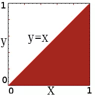

 satisfies Laplace’s equation in three dimensions everywhere in space that there is no electric charge.


 is a complex field, in the sense that it has both real and imaginary components, and we can… really imagine it. The equation can be decomposed into two equations, one for the real part and one for the complex part of
  , and we can plot it using a polar plot at each value of x. Again, the equation is local and says that the curvature is what matters. Where the curvature of the real part is positive, the imaginary part will grow. Where the curvature of the imaginary part is positive, the real part will shrink. If initially the field looks like a plane wave
  where
where  is a constant, the equation is telling us the corkscrew will turn.
 is essentially the quantity that, together with the probability
  , satisfies the continuity equation
  when
when  follows the Schrödinger equation. In one dimension it is
 and working through a little math we get an equation for the flow of that is much simpler to picture.
 which is saying that the probability current is just “flowing uphill” of the phase. That’s what the phase of a wave function has always meant, in case, like me, you weren’t told. This simpler version gives insight that might even be useful to a new wave of physics students.
 of the corkscrew increases constantly to the right, so our equation tells us there is uniform probability current to the right.
 and
and  . In the following, ignore the constant factors of
  which could be swallowed into the definition of the phase. The phase at a point x will decrease if it is sloped and it will increase due to curvature of A
  . Meanwhile the amplitude A at the point x decreases from phase curvature or from slopes
  . The probability increases from amplitude curvature (“smoothing out humps”) and decreases wherever the phase is sloped
  . Hope this helps you picture some quantum dynamics.
 is already a continuous field, but quantum field theory refers to more than single-particle quantum mechanics. Moreover, we know that two particles are described in quantum mechanics as a six-dimensional wavefunction, yet quantum field theory discusses quantum fields that permeate all of space, in only three dimensions. The purpose of this post is to briefly summarize the steps from single-body to many-body quantum mechanics, which clarifies these questions. We follow the canonical quantization method. The intended audience is someone familiar with quantum field theory calculations, but wanting a reminder of its meaning.
 -particle wavefunction is
  -dimensional. For instance, for
  , the wavefunction is written in position basis as
  where
where  is the 3-dimensional position of particle 1. Recall that, for two identical particles, only the phase of a wavefunction changes if two of the particles are permuted, and in fact we can accept as experimental fact that the wavefunction is either completely symmetric (bosons) or anti-symmetric (fermions) under permutation. Note that the wavefunction notation above makes reference to which particle is which, and so for identical particles there is extra, non-physical information in the above notation. In fact, the symmetry means that it has
  fewer distinct points in its domain than expected (i.e. than
  ). This suggests that there is actually a more elegant way to describe the state. The more efficient way is in the basis of occupation number, which does not distinguish which particle is occupying each 3D-location, only how much each position is occupied. This better basis for identical particles is called Fock space. The Fock space vector
  means that there is
  . Rather than position basis, these vectors are often written in wavevector basis, but for conceptualizing them at this point, we can remain in position space.
 and
and  . These operators create or annihilate a particle in the state
  . That is,
  adds one particle to the location
  . We can define the so-called field operators that create a particle in eigenstate
  as
as  .
. . They’re defined on 3-dimensional space, since they operate on M-dimensional Fock-space where M is the number of orthogonal multi-particle states that span the available space. These operator fields are free to fluctuate in magnitude. The operators operate on the current state of the fields. The background state is time-independent, and so all dynamics is in the field operators. (While the operators are the interesting, evolving quantities, they must ultimately be applied to the state to refer to the state of the system.) Commutation relations enforce the underlying quantization of the single-particle wavefunctions.